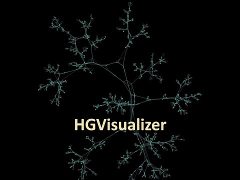
HGVisualizer is an interactive, real-time visualizer and simulator for evolving graphs (hypergraphs), inspired by the Wolfram Physics Project. The application allows you to define your own node-centric evolution rules, configure simulation parameters, and explore the emergent structure of dynamic graphs. Implements a spring-electrical embedding layout for clear and engaging visualization.
A hypergraph is a generalization of a graph where an edge (called a "hyperedge") can connect any number of nodes, not just two. The Wolfram Physics Project explores the idea that the universe can be modeled as a hypergraph, with simple local rules driving the evolution of the entire structure. In this project, we use a simplified (pairwise) version of these ideas to experiment with emergent complexity.
- User-defined evolution rules: Specify how nodes and edges evolve using a flexible rule system.
- Node-centric rule application: Rules are applied to nodes based on their local properties (e.g., edge count).
- Multiple operation types: Support for split, expand, merge, integrate, decay, and more.
- Interactive simulation controls: Pause, step, zoom, and pan the simulation.
- Configurable layout and simulation parameters: Adjust force-directed layout, damping, and more.
Rules in HGVisualizer are node-centric: each rule describes a condition on a node (such as the number of edges it has) and an operation to perform if the condition is met. Rules are evaluated for each node at every simulation step.
Each rule is specified on a single line in res/rules.config:
edges<=5 -> split(1)
edges==3 -> merge(2)
edges>7  -> expand(1)
Format:
<property><comparison><value> -> <operation>(<parameter>)
<property>: Currently onlyedgesis supported (number of edges connected to the node).<comparison>: One of<=,>=,==,!=,<,>.<value>: A positive integer.<operation>: One of the supported operation types (see below).<parameter>: A positive integer parameter for the operation.
| Operation | Example | Description |
|---|---|---|
split |
split(2) |
Clone the node into N new nodes, duplicating its edges. |
expand |
expand(1) |
For each of N edges, insert a new node in the middle (splitting the edge). |
merge |
merge(2) |
Merge up to N neighboring nodes into this node. |
integrate |
integrate(1) |
Connect the node to N second-tier neighbors (neighbors of neighbors). |
decay |
decay(1) |
Remove up to N edges from the node. |
expand_all |
expand_all(1) |
Expand all edges connected to the node. |
Note: The set of supported operations may grow in future versions.
Simulation and layout parameters are set in res/app.config.
Some parameters from previous versions have been removed or renamed.
Below are the currently supported parameters:
| Parameter | Description | Example Value |
|---|---|---|
layout.repulsion_constant |
Repulsion force constant for layout | 1.0 |
layout.attraction_constant |
Spring (edge) attraction constant | 0.1 |
layout.timestep |
Simulation time step | 1.0 |
layout.spring_length |
Desired spring (edge) length | 10.0 |
layout.damping_factor |
Damping factor for velocity | 0.9 |
layout.stablization_iterations |
Iterations per layout update | 100 |
model.updates_per_frame |
Number of model updates per frame | 1 |
| Key/Action | Effect |
|---|---|
TAB |
Toggle automatic model updates |
SPACE |
Pause/resume simulation |
N |
Toggle node rendering |
H |
Toggle highlight vertex mode |
| Mouse drag | Pan the view |
| Mouse wheel | Zoom in/out |
ESC |
Reset simulation |
- Edit
res/rules.configto define your evolution rules. - Edit
res/app.configto adjust simulation and layout parameters. - Build and run the application (see below).
- Use the controls above to interact with the simulation.
edges<=2 -> split(2)
edges==3 -> merge(1)
edges>5  -> decay(1)
edges>=4 -> integrate(2)
layout.repulsion_constant=1.0
layout.attraction_constant=0.1
layout.timestep=1.0
layout.spring_length=10.0
layout.damping_factor=0.95
layout.stablization_iterations=100
model.updates_per_frame=1
-
Dependencies:
- C++20 compiler
- SDL3
- SDL3_ttf
- NVIDIA CUDA Toolkit (for GPU-accelerated layout)
-
Build:
Use CMake:cmake -S . -B build cmake --build build -
Run:
./build/HGVisualizerApp
The goal of this tool is to aid in developing intuition for how structure might arise from a state with no predefined structure, and to explore the emergence of spontaneous complexity from the repeated application of simple rules. If we're going to explore the idea that the universe can be modeled as a graph, we need to recognize that even simple computational models, like graph rewriting systems, assume certain things: that there is something to rewrite, that it follows rules, and that some kind of ordering exists.
Thus, we are faced with a dilemma: if rules drive change, what determines the rules—and where and when they are applied? Do all possible rules exist? Do all possible events occur? If so, how does an embedded observer—who experiences definite events and a coherent reality—fit into this picture, and might the nature of the observer play a role in selecting or cohering that reality? As the developer of this tool, there is no external basis for determining which order or implementation is more correct—perhaps only the question: which of these resembles the universe as we, embedded from within, observe?
These questions lead us to a deeper challenge: how can we begin to model the origin of rules and order themselves? Does there exist a more fundamental explanation—one that doesn't begin with rules, entities, or space, but with the conditions that make anything possible at all? At its core, when we create nodes and place edges to signify relations, is this mirroring what the universe is fundamentally doing? It seems evident that the first "relation" arises when the void can be distinguished from itself—that the most basic prerequisite for structure is the introduction of a distinction. Could the universe itself unfold from nothing but the capacity to distinguish?
“To draw a distinction is to bring the world into being.” — G. Spencer-Brown
- Edge Creation reduces the overall path distance between nodes, effectively "pulling" nodes closer together in the network. This provides an analogue for the force of gravity in the model, as it increases connectivity and can lead to clustering or condensation of the graph structure.
- Edge Removal increases the overall path distance between nodes, effectively "pushing" nodes apart in the network. This acts as an analogue for an expanding universe, where the removal of connections can be seen as the creation of "new space" between regions of the graph, causing them to drift apart.
- Terminal States:
During the evolution, certain regions of the graph may reach a terminal state—a configuration in which no further rules can be applied to the nodes in that region. These terminal states can be interpreted as analogues of black holes or singularities in the model, representing areas where the local structure has become "frozen" and isolated from further evolution. This highlights how simple local rules can give rise to complex and emergent phenomena reminiscent of features in our universe. - Event Horizons:
As the graph evolves, it is possible for parts of the graph to become disconnected from the rest, forming isolated subgraphs. These disconnected regions can be thought of as analogues of event horizons—boundaries beyond which information or influence cannot propagate to the rest of the network. In cosmology, the cosmic event horizon is defined by the limits imposed by the speed of light and the expansion of the universe, beyond which events cannot affect an observer. Similarly, in the simulation, once a region becomes disconnected, it is causally isolated from the rest of the graph, and its evolution proceeds independently. This provides a conceptual parallel to the cosmic event horizon and highlights how local rules and edge dynamics can lead to emergent boundaries within the network. - Maximum Entropy:
The simulation can also explore states of maximum entropy, where the graph reaches a highly disordered or randomized configuration. In such a state, the connections between nodes are as uniformly distributed as possible, with no large-scale structure or clustering. This can be seen as an analogue to a universe in thermal equilibrium, where all distinctions between regions are erased and the system has reached its highest possible disorder.
This project is licensed under the GNU General Public License v3.0.
- Developed by Joe Mruz
HGVisualizer is an active work in progress. Feedback and contributions are welcome!